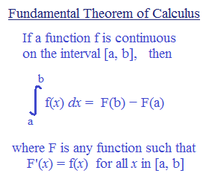
Let's talk about 7.3, in all its glory. This week we learned about solids of revolution, or taking the area under the curve and rotating it around a line to make a 3D shape. It's a pretty cool concept and I see how it could be applied to design and 3D printing, although there is probably a program that would accomplish this feat much faster and with more precision. The formal definition, as provided by Lamar University, is:
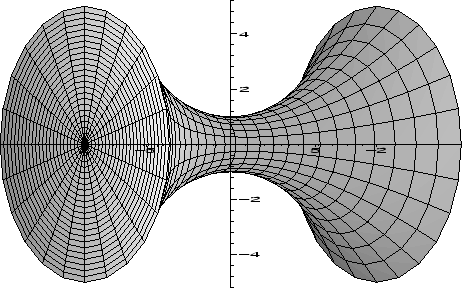
When we rotate a curve about a given axis to get the surface of the solid of revolution. It could be any vertical or horizontal axis, or a line.
So you got your function and you got your bounds and your are ready to revolve this puppy around a line. The easiest way to do this is to take pi * the integral from your bounds of f(x)^2 dx. It is similar to taking the 3D volume of a cylinder. It kind of uses the pi r ^2 equation but substituting the radius in for finding the area of the function under the curve due to the fluctuating equation and multiple radii.
The same method can be used around a vertical line like the y axis. The only difference is that you solve the equations for y (if not already provided) and use dy instead of dx. After changing your bounds to work for the y functions you are all good in the hood.
After recently completing the quiz, I feel as if I have learned this concept pretty well. I had to reteach some of it to myself as I went but overall I feel good about it. To prepare myself, I just had to listen to the way it was done in class and try a few on my own.


 RSS Feed